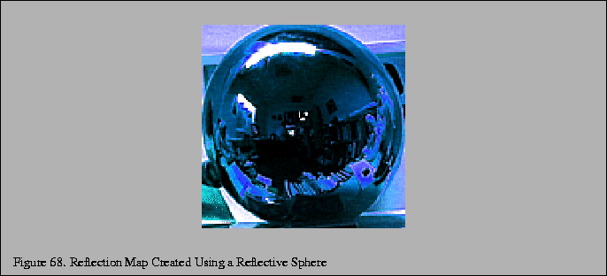
There are several ways to generate a specular sphere map. Two
physical approaches are worth mentioning. In the first approach, the
user literally takes a picture of a reflective sphere. Figure
68 was generated in this fashion. This technique is
problematic because the camera is visible in the sphere map. In
the second approach, a fisheye lens approximates the sphere mapping.
The problem with this technique is that no fisheye lens can provide
the
![]() field of view required for a correct result.
field of view required for a correct result.
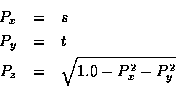
A sphere map can also be generated programmatically. Consider the
circle of the environment map within the square texture to be a unit
circle. For each point (s, t) in the unit circle, you can compute a
point ![]() on the sphere:
on the sphere:
The rays are intersected with the environment to determine the irradiance. A simple implementation of the algorithm is shown in the following pseudocode:
void gen_sphere_map(GLsizei width, GLsizei height, GLfloat pos[3],
                    GLfloat (*tex)[3])
{
  GLfloat ray[3], color[3], p[3], s, t;
  int i, j;

  for (j = 0; j < height; j++) {
    t = 2.0 * ((float)j / (float)(height-1) - .5);
    for (i = 0; i < width; i++) {
      s = 2.0 * ((float)i / (float)(width - 1) - .5);

      if (s*s + t*t > 1.0) continue;

      /* compute the point on the sphere (aka the normal) */
      p[0] = s;
      p[1] = t;
      p[2] = sqrt(1.0 - s*s - t*t);

      /* compute reflected ray */
      ray[0] = p[0] * p[2] * 2;
      ray[2] = p[1] * p[2] * 2;
      ray[3] = p[2] * p[2] * 2 - 1;
      fire_ray(pos, ray, tex[j*width + i]);
    }
  }
}
Note that you could easily optimize the routine such that the bounds on
i in the inner for loop were intelligently set based on
j.
The most interesting part of the computation has been encapsulated inside the fire_ray routine. fire_ray performs the ray/environment intersection given the starting point and the direction of the ray. Using the ray, it computes the color and puts the results into its third parameter (which is the appropriate location in the texture map).
A naive implementation such as the one above will lead to sampling artifacts. In reality, a texel in the image projects to a volume which should be intersected with the environment. To filter, you should choose several rays in this volume and combine the results.
The intersection and color computation can be done in several ways.
You can use a model of the scene and a ray tracing package.
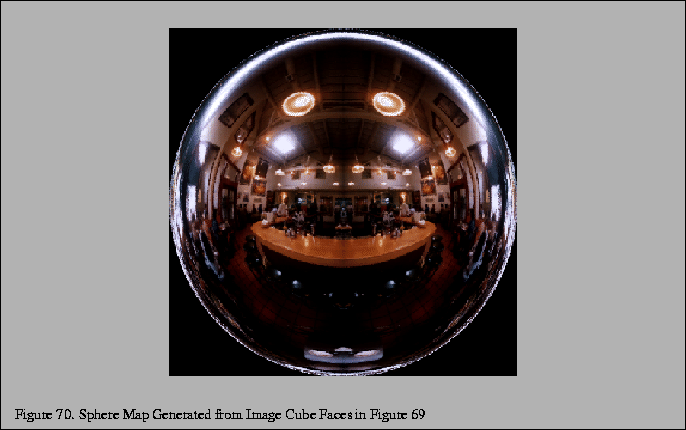
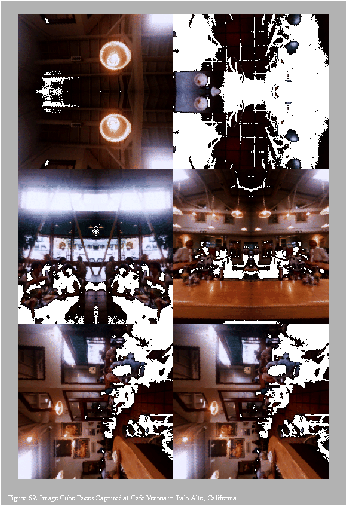
Alternately, you can represent the scene as six images which form the
faces of a cube centered around the point for which the sphere map is
being created. The images represent what a camera with a
![]() field of view and a focal point at the center of the square would see
in the given direction. The six images may be generated with OpenGL
or a rendering package, or can be captured with a camera.
Figure 69 shows six images which were acquired using a camera.
Once the six images have been acquired, the rays from the point are
intersected with the cube to provide the sphere map texel values.
Figure 70 shows the map generated from the cube faces
in Figure 69.
field of view and a focal point at the center of the square would see
in the given direction. The six images may be generated with OpenGL
or a rendering package, or can be captured with a camera.
Figure 69 shows six images which were acquired using a camera.
Once the six images have been acquired, the rays from the point are
intersected with the cube to provide the sphere map texel values.
Figure 70 shows the map generated from the cube faces
in Figure 69.